pacman::p_load(tidyverse, lubridate, arrow, sf)8 Location
Before counting or tracking devices, we must know where each device is. This chapter shows how to assign positions to WiFi detections, a foundational step that feeds into all downstream analyses.
WiFi sensors report detections, not coordinates: “device X was seen at time T with signal strength S.” When coverage areas overlap, the same device appears in multiple sensor logs simultaneously. Localization consolidates these scattered detections into a single position estimate per time window.
This requires two decisions:
- Temporal resolution: How often to update a device’s location? Every second captures fine-grained movement but amplifies noise; every minute smooths trajectories but misses quick stops.
- Spatial resolution: When multiple sensors detect the same device, which location to assign? Pick the strongest signal (Proximity), or compute a weighted average (Centroid).
8.1 Setup
Prepare data
Download our sample dataset to follow along, or use your own WiFi detection data: sample_loc.zip. The ZIP contains three files: wifi.parquet (WiFi detections for one device), gps.csv (GPS ground truth), and sensors.gpkg (sensor locations). Extract the ZIP into a working folder named sample_loc before running the code below. This GPS validation subset is the one dataset kept in a separate pseudonym space: its identifiers are keyed apart from the released data so participant GPS traces cannot be joined to the full dataset.
NoteAbout the sample dataset
Period: October 21 – November 14, 2019. A single device with paired GPS ground truth.
Location: UNIST campus, Ulsan, South Korea. 26 sensors in projected coordinates (KGD2002 Central Belt 2010): the 25 outdoor sensors plus one indoor sensor that detected this device. The toolkit’s main analyses use 24 of these positions (Appendix A).
Data structure:
| File | Rows | Columns |
|---|---|---|
wifi.parquet |
~86,000 | timestamp, source_address, sensor_name, rssi |
gps.csv |
~46,000 | source_address, timestamp, x, y |
sensors.gpkg |
26 | sensor_name, geom |
How we prepared this sample: historical selection and restricted export are implemented in scripts/0-4-unist19-location.R; downstream public re-pseudonymization is implemented in scripts/release/rekey_tutorial_data.py.
- Selected the device with most detections from the full dataset
- Exported the paired restricted WiFi and GPS records and sensor coordinates
- Replaced the retained restricted identifier in both public files with the same 32-character, release- and dataset-specific HMAC-SHA-256 pseudonym
This sample uses a single device with paired GPS ground truth, separate from the multi-device dataset used in later chapters (Count, Track, Revisits). Its 32-character pseudonym was assigned downstream when this tutorial archive was prepared for release.
Load packages and data
Load required packages using pacman::p_load(), which installs any missing packages automatically:
Load the data files:
sample_dir <- "sample_loc"  # folder containing the extracted ZIP
wifi_raw <- read_parquet(file.path(sample_dir, "wifi.parquet"))
gps <- read_csv(file.path(sample_dir, "gps.csv"), show_col_types = FALSE) |>
  mutate(timestamp = ymd_hms(timestamp))
sensors <- st_read(file.path(sample_dir, "sensors.gpkg"), quiet = TRUE)
Extract sensor coordinates for localization:
sensor_locations <- sensors |>
  mutate(
    x_sensor = st_coordinates(sensors)[, 1],
    y_sensor = st_coordinates(sensors)[, 2]
  ) |>
  st_drop_geometry()
TipPreview loaded data
WiFi data (probe request detections with signal strength):
head(wifi_raw, 3) timestamp source_address sensor_name rssi
1 2019-10-21 00:01:35 b84170e4d8f3f45a54ebc86352d8c5a4 comm_center -75
2 2019-10-21 00:01:36 b84170e4d8f3f45a54ebc86352d8c5a4 comm_center -75
3 2019-10-21 00:01:51 b84170e4d8f3f45a54ebc86352d8c5a4 comm_center -75timestamp: Detection time (second precision)source_address: 32-character lowercase release- and dataset-specific HMAC-SHA-256 pseudonym, consistent acrosswifi.parquetandgps.csvonly within this tutorial archivesensor_name: Which sensor detected this devicerssi: Signal strength in dBm (closer to zero = stronger signal)
Sensors (point geometries in projected coordinates):
head(sensor_locations, 3) sensor_name x_sensor y_sensor
1 bus_station 398694.9 332932.1
2 108_front_outs~ 398418.3 332757.7
3 206_front 398305.3 332761.08.2 Pipeline
The localization pipeline has three steps: create time windows, aggregate detections by sensor, and assign each window to a location. We use 20-second windows with Proximity (strongest signal wins); see Section 8.4 for the rationale.
Time windows
Group detections into fixed intervals. All detections within the same 20-second window will be aggregated together:
sampling_window <- 20  # seconds

wifi_windowed <- wifi_raw |>
  mutate(
    time_window = floor_date(timestamp, paste(sampling_window, "seconds"))
  )
Aggregate
Within each time window, aggregate detections per sensor. Each RSSI reading (negative dBm) is shifted by adding 100 to produce a positive score before summing, so that both more frequent and stronger detections yield a larger total:
wifi_aggregated <- wifi_windowed |>
  group_by(source_address, time_window, sensor_name) |>
  summarise(
    strength = sum(100 + rssi),
    n_detections = n(),
    .groups = "drop"
  ) |>
  left_join(sensor_locations, by = "sensor_name")
The strength column serves as the localization score: a sensor with many strong detections accumulates a higher total than one with few weak detections.
Assign location
Pick the sensor with strongest cumulative signal (Proximity method):
wifi_located <- wifi_aggregated |>
  arrange(source_address, time_window, desc(strength), sensor_name) |>
  distinct(source_address, time_window, .keep_all = TRUE) |>
  select(source_address, time_window, sensor_name, x_sensor, y_sensor)

head(wifi_located)
source_address time_window sensor_name x_sensor y_sensor
1 b84170e4d8f3f45a54ebc86352d8c5a4 2019-10-21 00:01:20 comm_center 398463.8 332750.2
2 b84170e4d8f3f45a54ebc86352d8c5a4 2019-10-21 00:01:40 comm_center 398463.8 332750.2
3 b84170e4d8f3f45a54ebc86352d8c5a4 2019-10-21 00:02:00 comm_center 398463.8 332750.2Each row is now one retained pseudonymous identifier assigned to one location for one time window. Ordering by sensor_name makes exact signal-score ties deterministic rather than dependent on input row order.
TipAlternative: Weighted Centroid
Proximity assigns devices to discrete sensor locations. If you need continuous coordinates for mapping or distance calculations, compute a weighted average of all detecting sensors:
wifi_centroid <- wifi_aggregated |>
  group_by(source_address, time_window) |>
  summarise(
    x_est = sum(x_sensor * strength, na.rm = TRUE) / sum(strength, na.rm = TRUE),
    y_est = sum(y_sensor * strength, na.rm = TRUE) / sum(strength, na.rm = TRUE),
    .groups = "drop"
  )
\[ x_{est} = \frac{\sum_{i} w_i \cdot x_i}{\sum_{i} w_i} \]
where \(w_i = 100 + RSSI_i\). The strength column is the per-sensor sum of these weights within each window.
8.3 Sensor spacing
Sensor spacing matters more than localization method. When sensors are too far apart, devices pass through gaps undetected, and no algorithm can compensate for missing data.
We tested this by progressively removing sensors from our campus deployment:
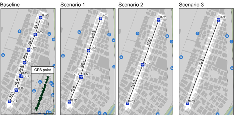
Detection holds to about 100m spacing and breaks down beyond it:
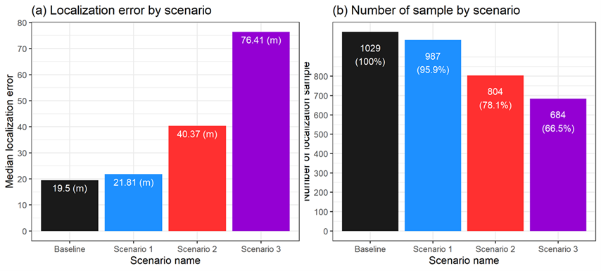
NoteInterpreting sensor spacing results
| Spacing | Sensors | Detection Rate |
|---|---|---|
| ~50m | 25 | 100% |
| ~100m | 12 | 96% |
| ~150m | 6 | 78% |
| ~320m | 4 | 67% |
The jump from 100m to 150m is where coverage breaks down. At ~50m spacing, every device was detected; halving the network to ~100m spacing still detected 96%. Beyond that, coverage degraded rapidly: at ~150m spacing, 22% of devices were missed entirely, and the localization error visible in the figure grew accordingly. These scenario figures come from the historical sensor-density experiment on this deployment and are shown for the coverage pattern rather than the exact error values.
Recommendation: Keep sensors within 100m of each other. If budget forces wider spacing, accept that you’ll miss significant pedestrian traffic, and counts will underestimate accordingly.
8.4 Method selection
Two parameters require decisions: time window length and localization method. Our validation uses GPS ground truth from multiple participants to compare approaches.
Time window
Window length trades off temporal resolution against estimation stability. Short windows (1–10s) capture fine-grained movement but produce noisy estimates; long windows (1–3min) yield stable estimates but blur movement patterns.
We tested windows from 1 to 120 seconds against GPS ground truth from 93 participants:
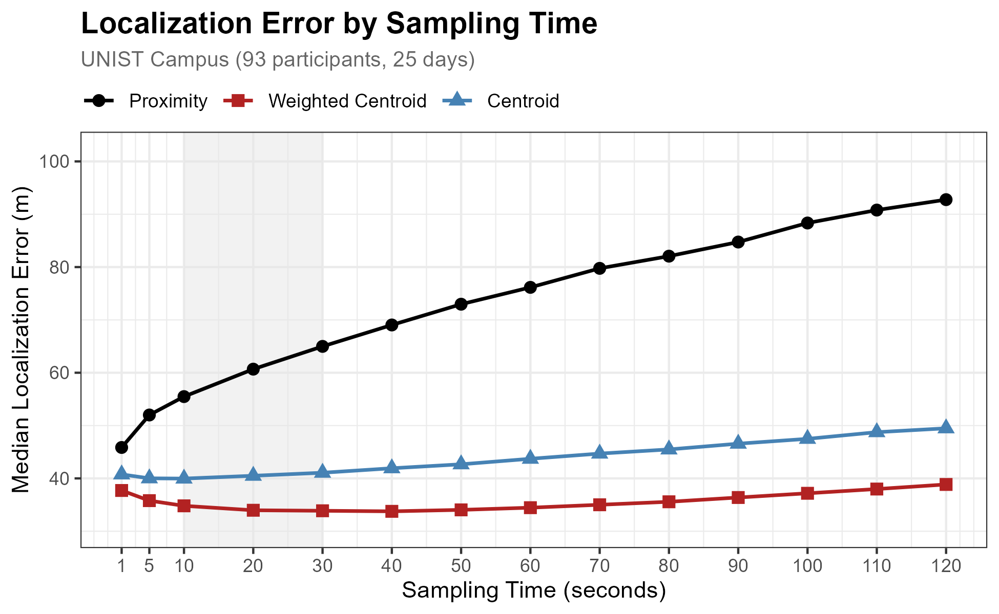
NoteInterpreting time window results
Weighted Centroid reaches the lowest median error (~34m around 20–30 second windows). Proximity tracks it closely, within about 2m across the 10–30 second band, and its own median error is lowest at exactly 20 seconds (~36m). Centroid trails at ~40m. All three methods degrade slowly at longer windows, as a single window increasingly blends detections from different positions.
We default to 20 seconds as a reasonable balance:
- Short enough to capture movement between locations
- Long enough to aggregate multiple detections for stable estimates
- Aligns well with typical pedestrian pace (~1.4 m/s = 28m in 20s)
- The GPS benchmark supports it directly: Proximity’s error is minimized there
Localization method
We use Proximity (assign to strongest sensor) for the pipeline in subsequent chapters:
- Output maps directly to a single sensor, essential for discrete analyses like counting at specific locations and building OD matrices between sensors
- Centroid and Weighted Centroid produce continuous coordinates that fall between sensors, which cannot be used for sensor-level counting or tracking
- At the adopted 20-second window, Proximity gives up very little accuracy (~36m vs ~34m median error), so the discrete output costs almost nothing
For applications requiring precise continuous positioning (e.g., indoor navigation), Weighted Centroid is the better choice.
NoteMore on localization methods
Li et al. (2021) categorize IoT localization methods by complexity and accuracy:
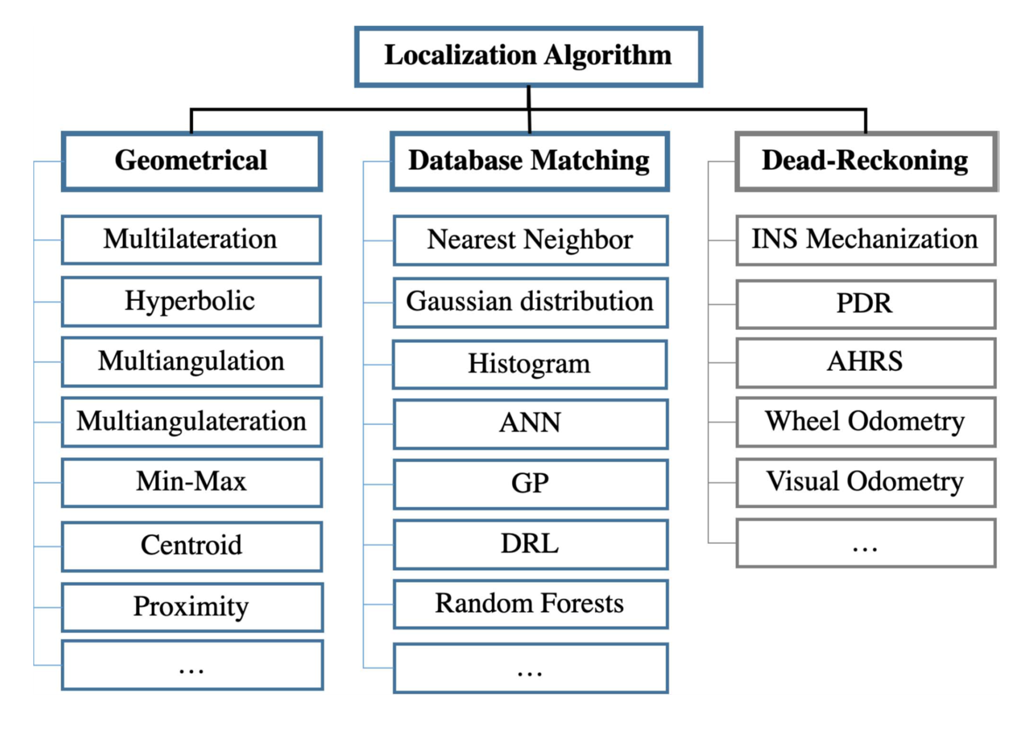
For low-cost outdoor deployments with sparse sensor networks, only Proximity and Centroid are practical. Methods requiring precise timing (ToA, TDoA) or dense arrays (fingerprinting) demand hardware beyond typical WiFi sensing setups.
Reference: Li, You, et al. Toward location-enabled IoT (LE-IoT). IEEE Internet of Things Journal, 2020, 8.6: 4035-4062.