8 Count

While Location identifies where devices are, Count answers how many. This chapter shows how to aggregate WiFi detections into device counts (by sensor, by hour, by day type) to estimate pedestrian activity across your study area.

The core metric is unique devices per time window: for each sensor and time period, count distinct MAC addresses. Temporal aggregation reveals daily rhythms; spatial aggregation reveals hotspots. Together, they characterize when and where people concentrate.

8.1 Setup

Prepare data

Download our sample dataset to follow along, or use your own WiFi detection data: sample_main.zip. The ZIP contains three files: wifi.parquet (WiFi detections), sensors.gpkg (sensor locations), and poi.gpkg (campus landmarks).

About the sample dataset

Period: October 28 – November 3, 2019 (one week). Includes a campus interview event (Nov 1–2) and the start of a school festival (Nov 3).

Location: UNIST campus, Ulsan, South Korea. 24 outdoor sensors covered dormitories, academic buildings, cafeteria, library, gym, and bus station.

Data structure:

File	Rows	Columns
`wifi.parquet`	~4.2M	`timestamp`, `source_address`, `sensor_name`, `rssi_median`, `rssi_sum`, `n`, `detections`
`sensors.gpkg`	24	`sensor_name`, `geom`
`poi.gpkg`	6	`name`, `geom`

How we prepared this sample (see scripts/0-3-unist19-prep.R):

Removed randomized MACs (locally-administered bit), stationary devices, and devices with fewer than 5 detections
Hashed remaining MAC addresses (SHA-256, first 12 characters) for privacy
Aggregated to 20-second windows with median RSSI and detection counts
Exported as Parquet for efficient storage

Load packages and data

Load required packages using pacman::p_load(), which installs any missing packages automatically:

pacman::p_load(tidyverse, lubridate, arrow, sf, ggmap, ggrepel)

Load the data files:

wifi_raw <- read_parquet("../workflow/unist19_main/data/wifi.parquet")
sensors <- st_read("../workflow/unist19_main/data/sensors.gpkg", quiet = TRUE)
poi <- st_read("../workflow/unist19_main/data/poi.gpkg", quiet = TRUE)

Preview loaded data

WiFi data (20-second aggregated detections):

head(wifi_raw, 3)

            timestamp source_address       sensor_name rssi_median rssi_sum   n detections
1 2019-10-28 00:00:00   014ca1637458     PC_room_front       -76.5    -1371  61         18
2 2019-10-28 00:00:00   02f35e3b75cf football_field_front    -65.0     -461 132          7
3 2019-10-28 00:00:00   03cac8c223f6          202_back       -74.0      -74   2          1

timestamp: Start of 20-second aggregation window
source_address: SHA-256 hashed device identifier (first 12 characters)
sensor_name: Which sensor detected this device
rssi_median: Median signal strength in dBm within the window
rssi_sum: Cumulative signal strength (sum of RSSI values)
n: Total raw packets captured
detections: Number of 1-second slots with at least one detection

Sensors (point geometries with location coordinates):

head(sensors, 3)

Simple feature collection with 3 features and 1 field
Geometry type: POINT
Geodetic CRS:  WGS 84
      sensor_name                      geom
1     bus_station POINT (129.1918 35.57348)
2 108_front_outs~ POINT (129.1887 35.57197)
3        112_side  POINT (129.187 35.57127)

8.2 Pipeline

Hourly counts

Aggregate detections into hourly counts by counting unique devices across all sensors:

hourly_counts <- wifi_raw |>
  mutate(
    hour = floor_date(timestamp, "hour"),
    day_type = if_else(wday(timestamp) %in% c(1, 7), "Weekend", "Weekday")
  ) |>
  group_by(hour, day_type) |>
  summarise(n_devices = n_distinct(source_address), .groups = "drop")

head(hourly_counts)

# A tibble: 6 x 3
  hour                day_type n_devices
  <dttm>              <chr>        <int>
1 2019-10-28 00:00:00 Weekday       1316
2 2019-10-28 01:00:00 Weekday       1192
3 2019-10-28 02:00:00 Weekday       1100
4 2019-10-28 03:00:00 Weekday       1035
5 2019-10-28 04:00:00 Weekday        982
6 2019-10-28 05:00:00 Weekday       1008

The day_type column distinguishes weekday from weekend patterns. University campuses show pronounced differences between the two.

Average daily pattern

Collapse across days to compute the typical hourly rhythm:

hourly_pattern <- hourly_counts |>
  mutate(hour_of_day = hour(hour)) |>
  group_by(hour_of_day, day_type) |>
  summarise(
    mean_devices = mean(n_devices),
    sd_devices = sd(n_devices),
    .groups = "drop"
  )

8.3 Temporal patterns

Plot the average hourly pattern with standard deviation bands:

ggplot(hourly_pattern, aes(x = hour_of_day, y = mean_devices,
                           color = day_type, fill = day_type)) +
  geom_ribbon(aes(ymin = pmax(0, mean_devices - sd_devices),
                  ymax = mean_devices + sd_devices),
              alpha = 0.2, color = NA) +
  geom_line(linewidth = 1) +
  geom_point(size = 2) +
  scale_x_continuous(breaks = seq(0, 23, by = 3)) +
  scale_color_manual(values = c("Weekday" = "#2c7bb6", "Weekend" = "#d7191c")) +
  scale_fill_manual(values = c("Weekday" = "#2c7bb6", "Weekend" = "#d7191c")) +
  labs(x = "Hour of Day", y = "Unique Devices Detected", color = NULL, fill = NULL) +
  theme_bw()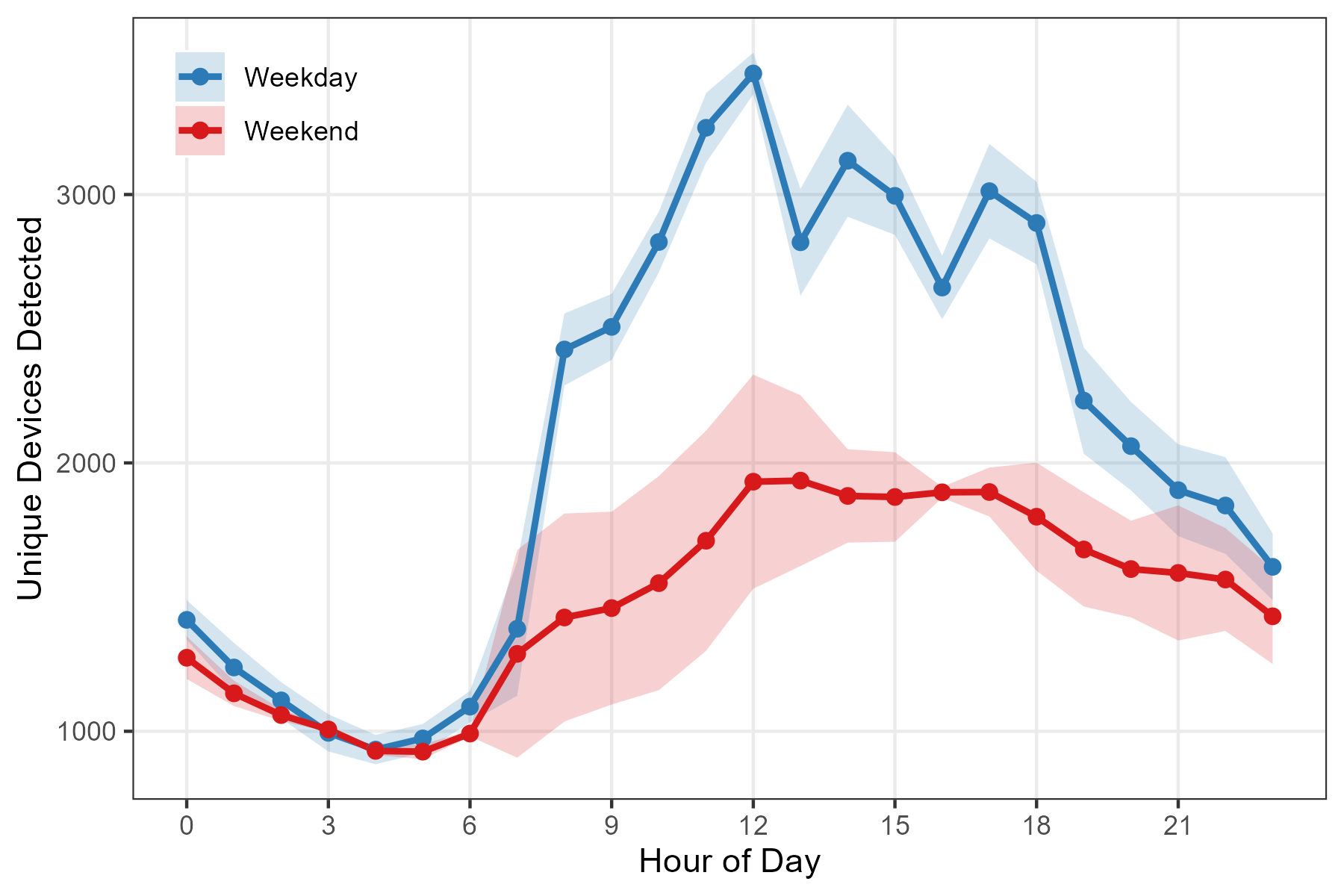

**Hourly pattern by day type.** Shaded bands show +/- 1 standard deviation.

Interpreting the temporal pattern

The weekday curve shows a clear work schedule: activity ramps up sharply after 7am, peaks at noon (~3,500 devices per hour during the lunch rush), and remains elevated through the afternoon until tapering after 7pm. Weekends are flatter, peaking around midday–afternoon at ~1,950 devices, roughly half the weekday peak.

Key observations:

Peak timing: Weekdays peak at noon (lunch hour); weekends show a broader plateau from noon to early evening
Morning ramp: Weekdays show steep 7-9am increase (commute arrival); weekends rise gradually
Evening decay: Both patterns decline after 7pm, but weekends maintain relatively higher late-night activity

Calendar view

A calendar-style small multiples plot reveals day-to-day variability. Special events or weather disruptions appear as anomalies against the regular rhythm.

daily_hourly <- wifi_raw |>
  mutate(
    date = as.Date(timestamp),
    hour_of_day = hour(timestamp)
  ) |>
  group_by(date, hour_of_day) |>
  summarise(n_devices = n_distinct(source_address), .groups = "drop")

ggplot(daily_hourly, aes(x = hour_of_day, y = n_devices)) +
  geom_line(linewidth = 0.5) +
  facet_wrap(~ date, ncol = 7, scales = "free_y") +
  labs(x = "Hour", y = "Devices") +
  theme_minimal()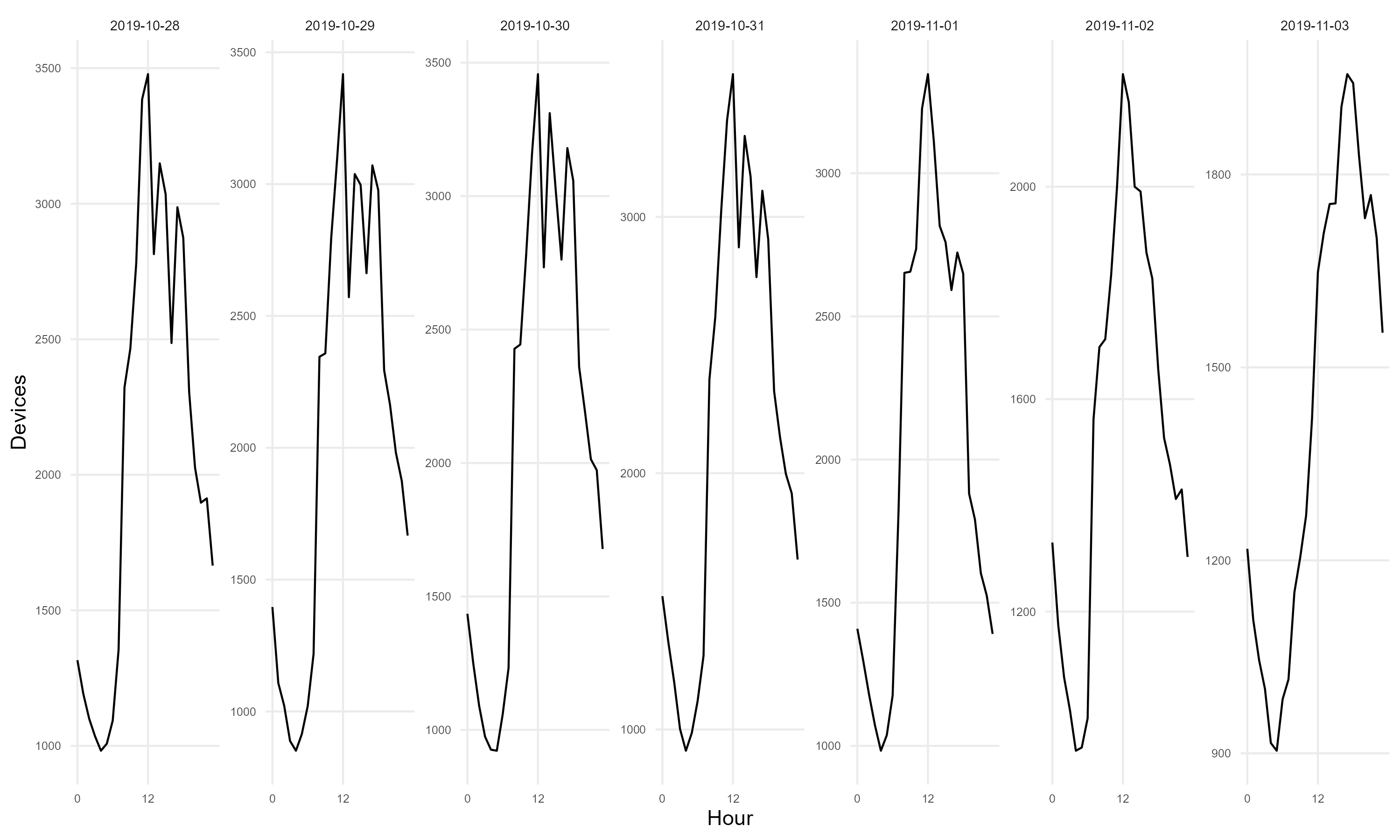

Calendar view: each panel shows one day’s hourly pattern.

The calendar view reveals which days deviate from the typical pattern. Campus events or holidays become visible as unusual curves among the regular rhythm.

8.4 Spatial patterns

Counts vary by location. Some sensors cover high-traffic corridors; others monitor quieter areas. Mapping counts by sensor reveals spatial hotspots.

Sensor-level aggregation

Count unique devices per sensor, filtering to midday hours (11am–3pm) when activity is most consistent:

sensor_counts <- wifi_raw |>
  mutate(
    day_type = if_else(wday(timestamp) %in% c(1, 7), "Weekend", "Weekday"),
    hour_of_day = hour(timestamp)
  ) |>
  filter(hour_of_day >= 11 & hour_of_day <= 14) |>
  group_by(sensor_name, day_type) |>
  summarise(n_devices = n_distinct(source_address), .groups = "drop")

Map visualization

Join counts with sensor coordinates and plot on a basemap. Circle size encodes device count:

sensors_with_counts <- sensors |>
  left_join(sensor_counts, by = "sensor_name")

ggmap(base_map, darken = c(0.3, "white")) +
  geom_sf(data = sensors_with_counts, aes(size = n_devices),
          color = "#d7191c", alpha = 0.85, inherit.aes = FALSE) +
  scale_size_continuous(range = c(1, 8), name = "Devices") +
  facet_wrap(~ day_type) +
  theme_bw() +
  theme(axis.title = element_blank(), axis.text = element_blank(), axis.ticks = element_blank())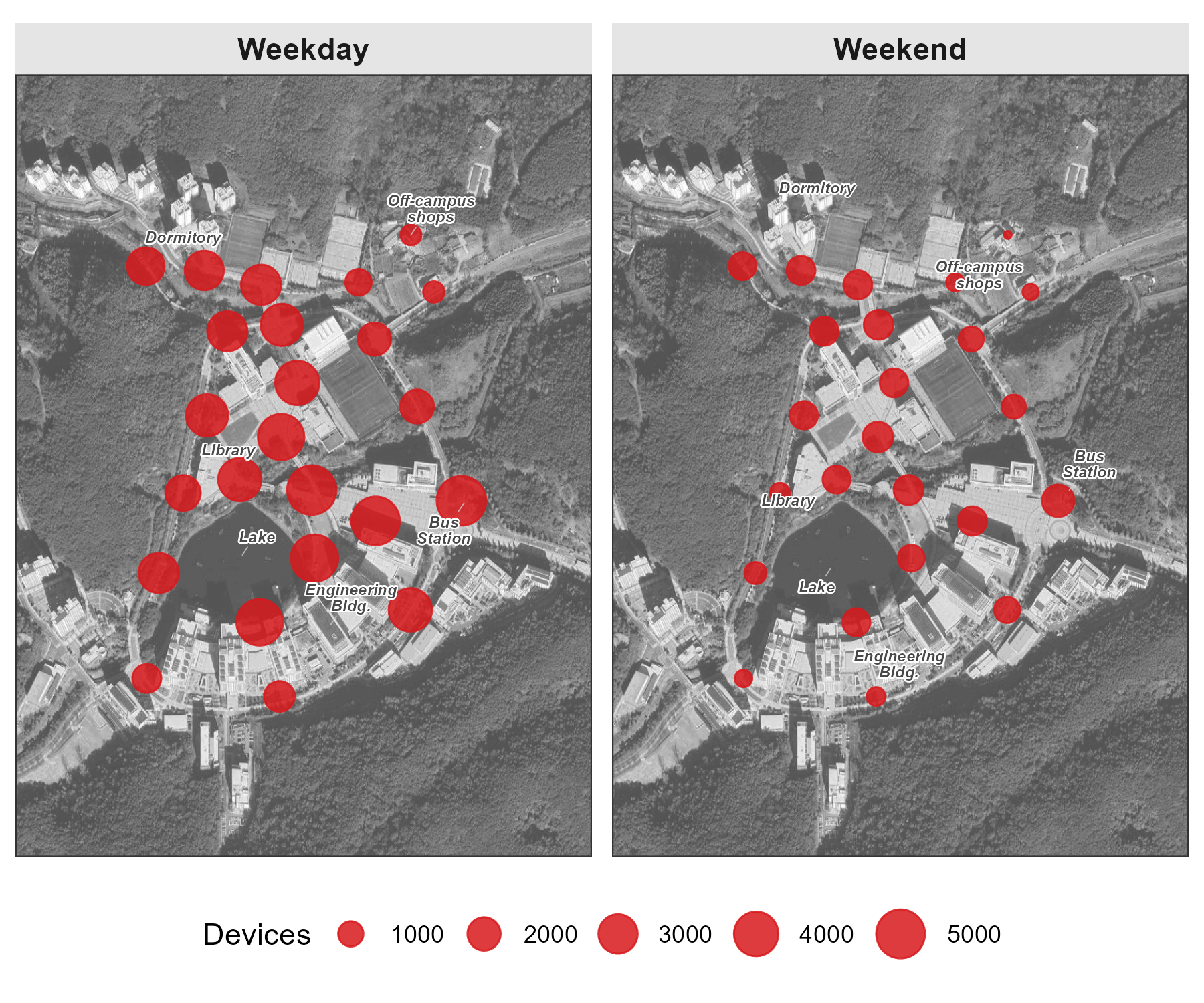

Sensor counts during midday (11:00–14:00), weekday vs weekend.

Interpreting the spatial pattern

The spatial contrast reveals functional zones:

Dormitory sensors: Similar counts on weekdays and weekends (residents are present regardless of schedule)
Engineering building sensors: Pronounced weekday peaks (students commute for classes then disperse)
Cafeteria sensors: High traffic on both day types, but weekday lunch crowds are larger
Bus station: Strong weekday presence as commuters arrive and depart; quieter on weekends

The map shows how different campus zones serve different functions: residential areas maintain steady occupancy while academic areas pulse with the class schedule.

8.5 Note on MAC randomization

Modern mobile devices randomize their MAC addresses for privacy, generating multiple identifiers per person. Left uncorrected, this inflates device counts: one person can appear as several.

Our sample dataset addresses this at the preprocessing stage: randomized MACs are identified by the locally-administered bit and removed before hashing (see scripts/0-3-unist19-prep.R). The counts in this chapter therefore reflect only non-random, manufacturer-assigned addresses.

How random MACs are identified

The second character of a MAC address indicates whether it is locally administered (random) or globally unique (manufacturer-assigned):

# Applied to raw (unhashed) MAC addresses during preprocessing:
is_random_mac <- function(mac) {
  second_char <- substr(tolower(mac), 2, 2)
  second_char %in% c("2", "3", "6", "7", "a", "b", "e", "f")
}

Once MAC addresses are hashed, the original bit structure is lost. Filtering must happen before hashing.

Limitations of removal-based filtering

Removing random MACs is a conservative strategy: it eliminates inflated counts but also discards detections from modern devices that exclusively use randomized addresses. Counts therefore represent a lower bound on actual pedestrian presence.

In controlled environments (campus WiFi, events with registered devices), the non-random share tends to be higher and this approach works well. In public spaces where most devices randomize, consider ratio-based correction or supplementary data sources for calibration.