pacman::p_load(tidyverse, lubridate, arrow, sf, ggmap, ggrepel)10 Track
While Count summarizes observed presence, Track links successive locations of the same retained pseudonymous identifier. This chapter builds origin–destination (OD) matrices and flow maps that reveal recurring observed sensor-to-sensor flows across a study area.
The core concept is the trajectory: a sequence of localized observations for one retained identifier, bounded by gaps of inactivity. In this campus example, a gap of more than 30 minutes starts a new trajectory. Its first and last observed sensors define an OD pair. Aggregating these pairs reveals which observed sensor-to-sensor flows dominate and how they shift by time of day or day of week.
10.1 Setup
Prepare data
Download our sample dataset to follow along, or use your own WiFi detection data: sample_main.zip. The ZIP contains three files: wifi.parquet (WiFi detections), sensors.gpkg (sensor locations), and poi.gpkg (campus landmarks). Extract the ZIP into a working folder named sample_main before running the code below. The sample is a one-week filter of the released campus dataset, with the same pseudonyms and schema, so anything observed here can be followed into the full data. Timestamps are stored in UTC as in the release; the load step converts them once to Asia/Seoul so dates and hours follow the local calendar.
NoteAbout the sample dataset
This chapter uses the same UNIST campus dataset introduced in Count: see that chapter for the period, sensor coverage, schema, and preparation steps.
Load packages and data
The code blocks below are displayed rather than executed when the book is rendered. scripts/4-4-track.R runs the same steps end to end.
Load required packages using pacman::p_load(), which installs any missing packages automatically:
Load the data files. The public file ships without the strength_sum localization score, so we restore it right away, the toolkit’s convention for public files:
sample_dir <- "sample_main"  # folder containing the extracted ZIP
wifi_raw <- read_parquet(file.path(sample_dir, "wifi.parquet")) |>
  mutate(
    timestamp = with_tz(timestamp, "Asia/Seoul"),
    strength_sum = 100 * detections + rssi_sum
  )
sensors <- st_read(file.path(sample_dir, "sensors.gpkg"), quiet = TRUE)
poi <- st_read(file.path(sample_dir, "poi.gpkg"), quiet = TRUE)
Configure basemap
Flow maps overlay movement data on a geographic basemap. Choose one of these options:
For satellite imagery, register a Google Maps API key:
register_google(key = "YOUR_API_KEY")

bbox <- st_bbox(sensors)
base_map <- get_map(
  location = c(lon = mean(bbox[c(1,3)]), lat = mean(bbox[c(2,4)])),
  zoom = 16, maptype = "satellite", source = "google"
)
For a free alternative (no API key required):
bbox <- st_bbox(sensors)
base_map <- get_stadiamap(
  bbox = c(left = bbox["xmin"], bottom = bbox["ymin"],
           right = bbox["xmax"], top = bbox["ymax"]),
  zoom = 16, maptype = "stamen_toner_lite"
)
Extract sensor coordinates for plotting:
sensor_coords <- sensors |>
  st_coordinates() |>
  as_tibble() |>
  bind_cols(sensors |> st_drop_geometry() |> select(sensor_name))
TipPreview loaded data
WiFi data (20-second aggregated detections):
head(wifi_raw, 3) timestamp source_address sensor_name rssi_median rssi_sum detections strength_sum
1 2019-10-28 00:00:00 058d412bd4c8729dfad1d924006c7e06 108_front_outside -69 -69 1 31
2 2019-10-28 00:00:00 058d412bd4c8729dfad1d924006c7e06 bridge_main_engineer -73 -73 1 27
3 2019-10-28 00:00:00 1063540d3c6c1dd7492972f2d16a2760 203_front -64 -64 1 36timestamp: Start of 20-second aggregation windowsource_address: 32-character lowercase release- and dataset-specific HMAC-SHA-256 pseudonym; values match the released campus dataset, so sample observations can be followed into the full datasensor_name: Sensor that retained the aggregated observationrssi_median: Median signal strength in dBm within the windowrssi_sum: Sum of raw RSSI values (negative dBm) within the windowdetections: Number of 1-second slots with at least one detectionstrength_sum: Localization score, equal tosum(100 + RSSI)across the window’s detections; restored in the load step above as100 * detections + rssi_sum
Sensors (point geometries with location coordinates):
head(sensors, 5)Simple feature collection with 5 features and 1 field
Geometry type: POINT
Geodetic CRS: WGS 84
sensor_name geom
1 bus_station POINT (129.1918 35.57348)
2 108_front_outside POINT (129.1887 35.57197)
3 112_side POINT (129.187 35.57127)
4 104_back POINT (129.191 35.57212)
5 108_back POINT (129.189 35.57104)POI (reference labels for the map):
poiSimple feature collection with 6 features and 1 field
Geometry type: POINT
Geodetic CRS: WGS 84
name geom
1 Dormitory POINT (129.1878 35.57708)
2 Library POINT (129.1879 35.5738)
3 Bus Station POINT (129.1919 35.57353)
4 Engineering Bldg. POINT (129.1897 35.57187)
5 Off-campus shops POINT (129.191 35.57656)
6 Lake POINT (129.1884 35.57273)10.2 Pipeline
Localize
Each retained identifier-window may contain observations from multiple sensors. Before building trajectories, select one sensor at each timestamp using strength_sum = sum(100 + RSSI) and break exact score ties by sensor_name:
wifi <- wifi_raw |>
  arrange(source_address, timestamp, desc(strength_sum), sensor_name) |>
  distinct(source_address, timestamp, .keep_all = TRUE) |>
  select(source_address, timestamp, sensor_name)
This reduces the dataset from about 4.2 million rows to about 2.7 million by keeping one deterministic sensor assignment per identifier-window.
Define trajectories
Segment the localized observations into trajectories. For each retained identifier, calculate the time gap between consecutive observations. When the gap exceeds 30 minutes, start a new trajectory:
gap_threshold <- 30  # minutes

trajectories <- wifi |>
  arrange(source_address, timestamp) |>
  group_by(source_address) |>
  mutate(
    time_gap = as.numeric(difftime(timestamp, lag(timestamp), units = "mins")),
    new_trajectory = is.na(time_gap) | time_gap > gap_threshold,
    trajectory_id = cumsum(new_trajectory)
  ) |>
  ungroup()
Extract OD pairs
For each trajectory, extract the first and last observed sensors. Exclude trajectories with identical endpoints or fewer than two localized observations:
od_pairs <- trajectories |>
  group_by(source_address, trajectory_id) |>
  summarise(
    origin = first(sensor_name),
    destination = last(sensor_name),
    trajectory_start = min(timestamp),
    trajectory_end = max(timestamp),
    n_detections = n(),
    .groups = "drop"
  ) |>
  filter(
    origin != destination,
    n_detections >= 2
  )
Build OD matrix
Count trajectory segments between each endpoint pair and compute their within-origin shares. This creates an OD matrix of observed first-to-last sensor pairs:
od_counts <- od_pairs |>
  count(origin, destination, name = "n_segments")

od_probs <- od_counts |>
  group_by(origin) |>
  mutate(
    total_from = sum(n_segments),
    prob = n_segments / total_from
  ) |>
  ungroup()

od_probs |>
  filter(origin == "104_back") |>
  arrange(desc(n_segments)) |>
  head(3)
# A tibble: 3 x 5
origin destination n_segments total_from prob
<chr> <chr> <int> <int> <dbl>
1 104_back bus_station 1691 5001 0.338
2 104_back bridge_main_engineer 388 5001 0.078
3 104_back 108_back 383 5001 0.077Among qualifying segments whose first sensor is 104_back, 34% end at bus_station and 8% at bridge_main_engineer. These are endpoint shares, not mode-specific travel probabilities.
10.3 Flow map
Flow maps display observed OD pairs on a geographic basemap, with arrows showing endpoint direction and line thickness encoding segment count.
Select the top OD pairs and join with sensor coordinates:
top_n <- 5

edges_top <- od_probs |>
  slice_max(n_segments, n = top_n) |>
  left_join(sensor_coords, by = c("origin" = "sensor_name")) |>
  rename(x_from = X, y_from = Y) |>
  left_join(sensor_coords, by = c("destination" = "sensor_name")) |>
  rename(x_to = X, y_to = Y)

edges_top |> select(origin, destination, n_segments)
# A tibble: 5 x 3
origin destination n_segments
<chr> <chr> <int>
1 btw_201_102 bus_station 2646
2 104_back bus_station 1691
3 lake 108_front_outside 1234
4 108_front_outside lake 1203
5 bus_station btw_201_102 1189Plot the flow map with curved arrows. Three small touches make flows legible on a satellite basemap: a grey casing drawn slightly wider under each colored arrow separates it from the imagery, double-ring nodes (a white ring under a colored dot) keep sensors visible on any background, and a white halo behind each label does the same for text. Pre-scaling the widths ourselves (instead of mapping n_segments directly) lets the casing track the flow width while the legend still shows real segment counts:
# Get labels for sensors in top flows
od_sensors <- unique(c(edges_top$origin, edges_top$destination))
sensor_labels <- sensor_coords |>
  filter(sensor_name %in% od_sensors)

# Pre-scale widths: casing sits 0.7 wider than the colored flow
width_breaks <- c(1500, 2000, 2500)
edges_top <- edges_top |>
  mutate(w_main = scales::rescale(n_segments, to = c(0.5, 3)),
         w_out  = w_main + 0.7)

ggmap(base_map, darken = c(0.3, "white")) +
  geom_curve(data = edges_top,
             aes(x = x_from, y = y_from, xend = x_to, yend = y_to,
                 linewidth = w_out),
             color = "grey25", curvature = 0.3,
             arrow = arrow(length = unit(2, "mm"), type = "closed"),
             show.legend = FALSE) +
  geom_curve(data = edges_top,
             aes(x = x_from, y = y_from, xend = x_to, yend = y_to,
                 linewidth = w_main),
             color = "#2c7bb6", curvature = 0.3,
             arrow = arrow(length = unit(1.5, "mm"), type = "closed")) +
  scale_linewidth_identity(
    name   = "OD segments",
    breaks = scales::rescale(width_breaks,
                             from = range(edges_top$n_segments), to = c(0.5, 3)),
    labels = scales::comma(width_breaks),
    guide  = guide_legend(override.aes = list(color = "#2c7bb6"))) +
  geom_point(data = sensor_labels, aes(x = X, y = Y),
             size = 2.5, color = "white") +
  geom_point(data = sensor_labels, aes(x = X, y = Y),
             size = 2, color = "#2c7bb6") +
  geom_text_repel(data = sensor_labels, aes(x = X, y = Y, label = sensor_name),
                  size = 2.5, fontface = "bold.italic",
                  bg.color = "white", bg.r = 0.15) +
  theme_void()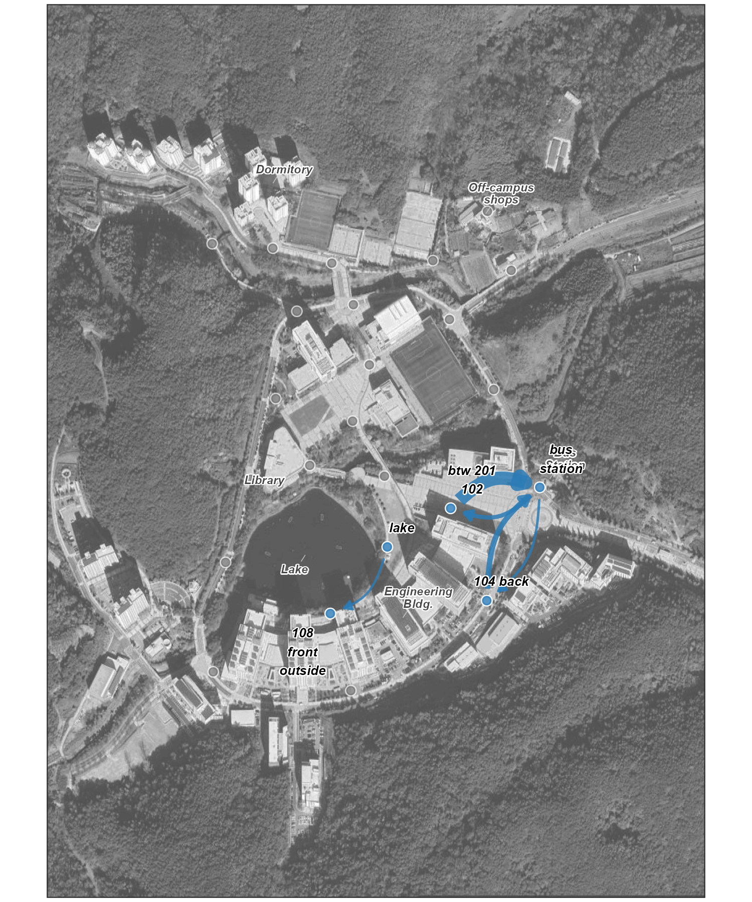
NoteReading the flow patterns
The largest endpoint counts involve the bus-station sensor:
- btw_201_102 → bus_station: 2,646 segments, the largest observed endpoint pair
- 104_back → bus_station: 1,691 segments
- lake ↔︎ 108_front_outside: 1,234 / 1,203 segments in the two directions
The reverse bus_station → btw_201_102 pair contains 1,189 segments. Known site functions provide context, but endpoint pairs do not reveal the exact route or travel mode.
10.4 Temporal patterns
Observed endpoint patterns vary by time. The same OD pairs can be grouped by weekday/weekend or by morning/evening to describe temporal contrasts.
Weekday vs Weekend
Split OD pairs by day type to compare weekday and weekend segment counts:
od_by_daytype <- od_pairs |>
  mutate(day_type = if_else(wday(trajectory_start) %in% c(1, 7),
                            "Weekend", "Weekday")) |>
  count(origin, destination, day_type, name = "n_segments")

# Top 3 endpoint pairs per day type
od_by_daytype |>
  group_by(day_type) |>
  slice_max(n_segments, n = 3)
# A tibble: 6 x 4
day_type origin destination n_segments
<chr> <chr> <chr> <int>
1 Weekday btw_201_102 bus_station 2104
2 Weekday 104_back bus_station 1398
3 Weekday bus_station btw_201_102 1025
4 Weekend btw_201_102 bus_station 542
5 Weekend dorm_front bus_station 303
6 Weekend 104_back bus_station 293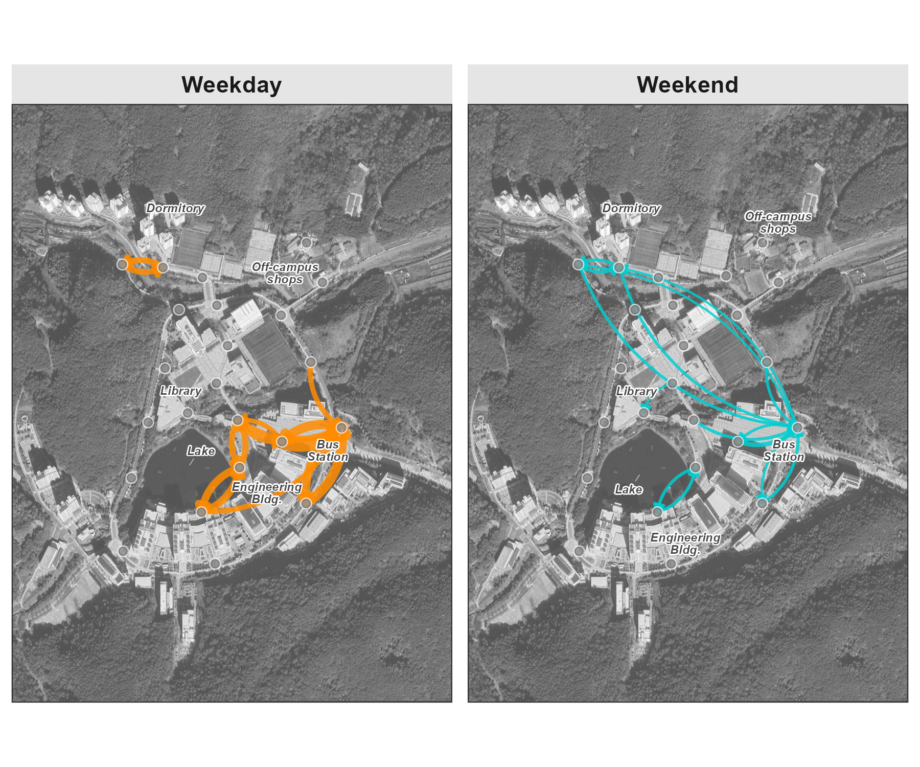
NoteWeekday vs Weekend differences
- Volume: the largest weekday pair contains 2,104 segments, 3.9 times the largest weekend pair (542)
- Bus-station endpoint: several leading pairs end at
bus_stationon both day types - Dormitory-area endpoints:
dorm_front → bus_stationrises to second on weekends, andparking_dorm → bus_stationenters the weekend top set - Lake-area endpoint:
108_front_outside → lakeenters the weekend top five
These are rank and count changes among retained trajectories, not evidence of trip purpose or population composition.
Morning vs Evening
Compare weekday morning (7–10 AM) and evening (5–8 PM) flows to describe directional asymmetry:
od_time_period <- od_pairs |>
  filter(wday(trajectory_start) %in% 2:6) |>  # weekdays only
  mutate(
    hour = hour(trajectory_start),
    time_period = case_when(
      hour >= 7 & hour < 10 ~ "Morning (7-10)",
      hour >= 17 & hour < 20 ~ "Evening (17-20)",
      TRUE ~ NA_character_
    )
  ) |>
  filter(!is.na(time_period)) |>
  count(origin, destination, time_period, name = "n_segments")

# Top 3 endpoint pairs per time period
od_time_period |>
  group_by(time_period) |>
  slice_max(n_segments, n = 3)
# A tibble: 6 x 4
time_period origin destination n_segments
<chr> <chr> <chr> <int>
1 Evening (17-20) 104_back bus_station 481
2 Evening (17-20) btw_201_102 bus_station 449
3 Evening (17-20) 108_front_outside bus_station 246
4 Morning (7-10) bus_station 104_back 269
5 Morning (7-10) btw_201_102 bus_station 268
6 Morning (7-10) bus_station btw_201_102 218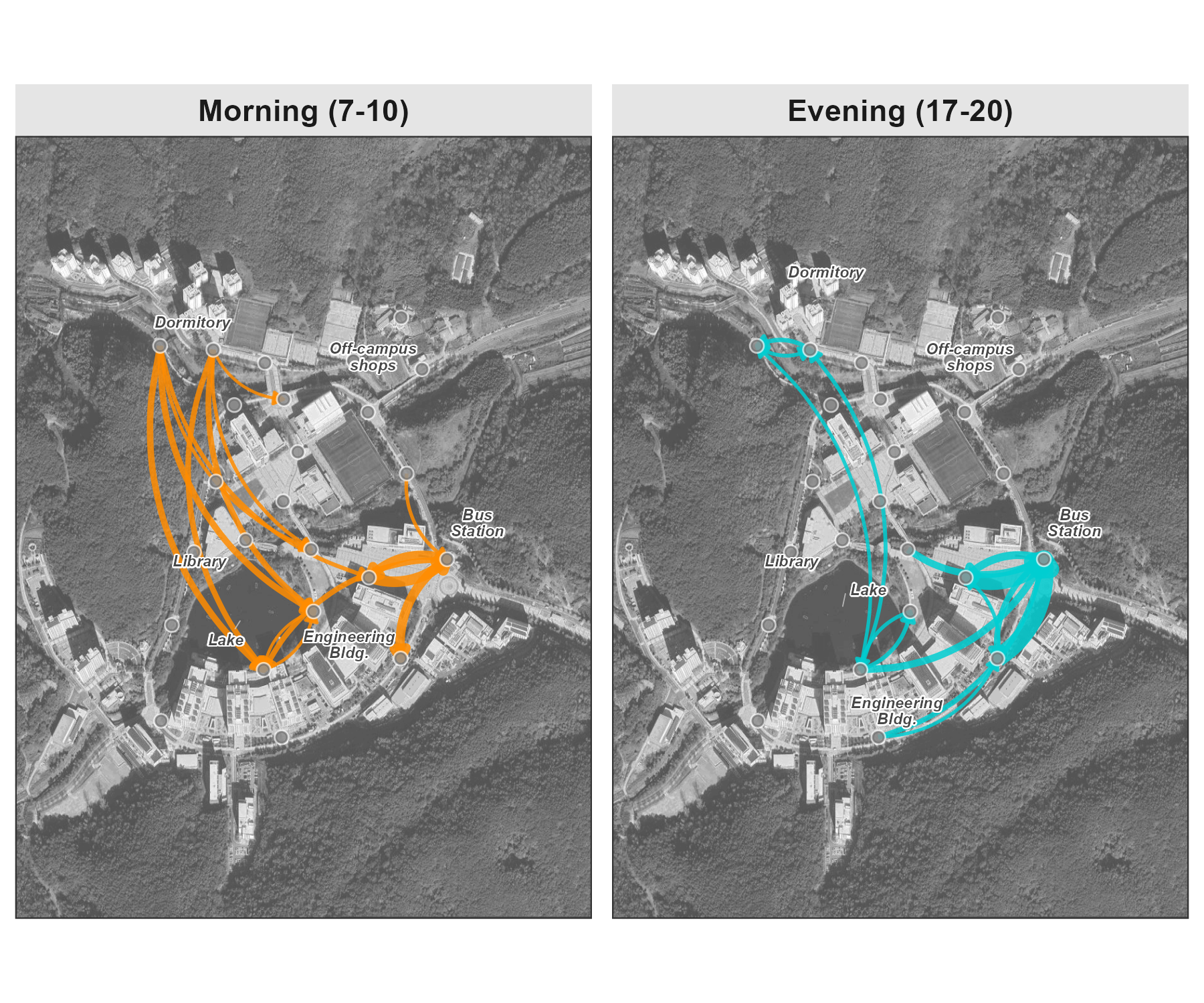
NoteMorning vs Evening asymmetry
The observed segments show directional asymmetry:
- Evening: the two largest pairs ending at
bus_stationcontain 481 and 449 segments - Morning:
bus_station → 104_backcontains 269 segments andbus_station → btw_201_102contains 218 - Direction: the leading evening pairs point toward
bus_station, while two leading morning pairs begin there
This timing is compatible with the documented campus schedule, but the observations do not identify students, travel mode, exact arrivals or departures, or individual commute behavior.
WarningInterpretation boundary
An OD pair is the first and last sensor assigned to a retained pseudonymous identifier within one threshold-defined trajectory. It is not a surveyed trip, an exact route, or proof of a person’s origin and destination. Coverage gaps, address filtering, sensor spacing, and the 30-minute threshold all shape the resulting flows.